Time complexity
How do we compare between two algorithms?
The first instinct would be to see which one is faster. So, we run two algorithms and see which one executes in lesser time. This won’t be the best judge because other factors like speed of computer, language, compiler, etc, come into play.
So, to compare we need a measurement of performance of an algorithm independent of these external factors.
Let’s think of the running time in some other way.
Runtime
The number of operations that run when executing an algorithm is it’s runtime. So, we calculate how many operations or steps an algorithm would take and the one with the lesser number of operations wins!
We choose the algorithm with lesser operations because we proved that the algorithm (the one with more operations) is doing unnecessary extra work when the same task can be done in lesser operations.
factorial = 1; #initial step
for i in range(1, n + 1): #for-step
    factorial *= i;  #step
It would take $2n + 1$ steps/operations to calculate the factorial of a number $n$. How?
initial step: Initializingfactorialis 1 operationstep: 1 operation running $n$ timesfor-step: Initializingiis 1 operation + $n - 1$ times incrementing it’s value = $n$ operations
Which gives $1 + (n * 1) + n = (2n + 1)$ operations.
Let’s see how long an algorithm takes to run in terms of the size of the input and growth with increase in input size.
1. Size of the input:
When calculating factorial in above example, for $n$ inputs it takes $2n + 1$ operations. For example, for $n = 10$, it takes 21 operations.
So, we think of the runtime of the algorithm as a function of the size of it’s input.
More input, more operations run, more work, higher runtime.
2. Growth with increase in input size:
As the input size increases some part of the algorithm dominates over the less important part. We look for the order of growth of it’s runtime.
Example, runtime on input size $n$ takes $5n^2 + 100n + 300$ operations.
For input size $n = 10$, runtime = $500 + 1000 + 300$
For input size $n = 10^{2}$, runtime = $5 * 10^{4} + 10^{4} + 300$
For input size $n = 10^{3}$, runtime = $5 * 10^{6} + 10^{5} + 300$
For input size $n = 10^{4}$, runtime = $5 * 10^{8} + 10^{6} + 300$
The $5n^2$ term becomes larger than the remaining terms, $100n + 300$ , once $n$ becomes large enough, 20 in this case. We can say the runtime of this algorithm grows with order of $n^2$, dropping coefficient 6 and the remaining terms.
It doesn’t really matter what coefficient of $n^2$ terms is as long as for an equation $an^2 + bn + c$, there will always be values of $n$ for which $an^2$ term is much much greater than $bn + c$ terms.
When we drop the constant coefficients and the less significant terms, we use asymptotic notation.
Asymptotic notation
Also known as Bachmann–Landau notation, Asymptotic notations are the mathematical notations used to describe the running time of an algorithm when the input tends towards a particular value or a limiting value.
Let’s look at asymptotic notations for factorial example, where our runtime was $2n + 1$, so dropping the constant coefficients and the less significant terms, the significant part for our runtime would be $n$.
Some of it’s family members are:
- Theta notation $\Theta$
- Big-O notation $O$
- Omega notation $\Omega$
Let’s look at this linear search of a number target in an list of integers array
def linearSearch(target: int, array: [int], lenArray: int): # [4, 3, 8, 2]
    for i in range(lenArray): #[(0,4), (1, 3), (2, 8), (3, 2)]
        if array[i] == target:
            return index
    return -1
Tight Bounds: Theta
Tight bounds means that Big-$\Theta$ notation or Theta notation is like a range within which the actual time of execution of the algorithm will be.
Let’s look at our linearSearch function!
Say $c_1$ operations run in one iteration of the loop, $n$ is the number of times the loop will run ($n$ = lenArray), and other constant overhead operations (like return -1 and initializing i) are total $c_2$ operations.
Then, total time for linear search in the worst case is $c_1 * n + c_2$
As we learned for Asymptotic notations, we ignore the coefficients and the less significant terms, so runtime is $\Theta$(n). When we say the runtime of an algorithm is $\Theta(n)$, we’re saying when $n$ becomes large enough, runtime is at least $k_1 * n$ and at most $k_2 * n$.
Conclusion: The runtime $\Theta(f(n))$, for some function $f(n)$:
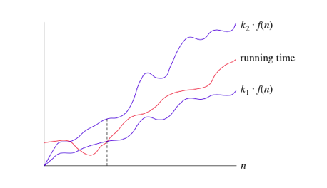
Once runtime gets large enough, the runtime is between $k_1 * f(n)$ and $k_2 * f(n)$.
When we use big-$\theta$ notation, we’re saying that we have an asymptotically tight bound on the running time. “Asymptotically” because it matters for only large values of n. “Tight bound” because we’ve nailed the running time to within a constant factor above and below.
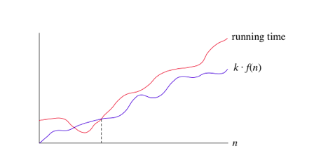
Upper Bounds: Big-O
This notation is known as the upper bound of the algorithm, or a Worst Case of an algorithm.
In our linearSearch function, the worst case would be that the target is not found in the array.
So, the Big-O would be $O(n)$.
When we say, for linear search the complexity is $\Theta(n)$, we mean that runtime as n increases is proportional to n, and by $O(n)$, we mean the time complexity will at most proportional to n.
If the running time is $\Theta(f(n))$, then it’s also $O(f(n))$. Converse is not necessarily true. Why? Because $O(f(n))$ is not always the time complexity of $f(n)$, just in the worst case.

We use big-O notation for asymptotic upper bounds, since it bounds the growth of the running time from above for large enough input sizes.
Lower Bounds: Omega
This notation is known as the lower bound of the algorithm, or a Best Case of an algorithm.
In our linearSearch function, the best case would be that the target is found at the first place in the array.
So, the Big-$\Omega$ would be $\Omega(1)$, i.e. constant time.
No matter how large the input of array is, if the element is always at the first place then the number of operations that will run will always be fixed amount.
Conclusion: If a runtime is $\Omega(f(n))$, then for larger enough $n$, the time complexity will be at least $k * f(n)$ for some constant $k$.
We use big-Ω notation for asymptotic lower bounds, since it bounds the growth of the running time from below for large enough input sizes.
Read more on Family of Bachmann–Landau notations
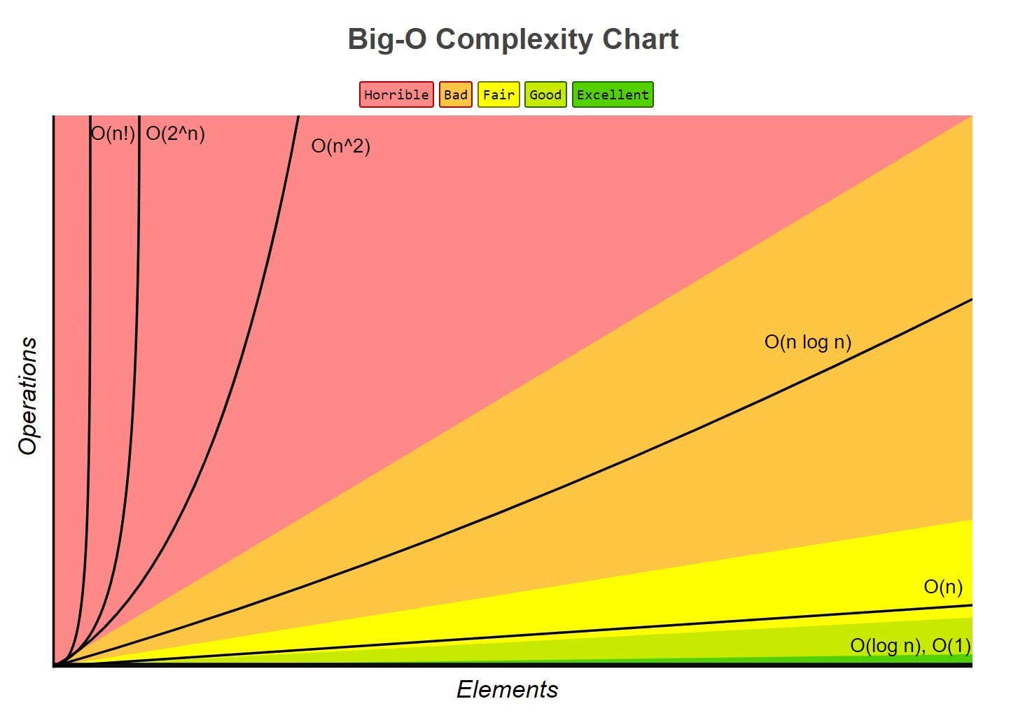
Functions in asymptotic notation
| Order of f | Name |
|---|---|
| 1 | Constant |
| $log n$ | Logarithmic |
| $n$ | Linear |
| $n * log n$ | Log Linear |
| $n^2$ | Quadratic |
| $2^n$ | Exponential |
| $n!$ | Factorial |
(in order of: fast to slow)
Constant Time $\Theta(1)$
When the number of operations are independent of the size of input, then the time complexity is constant.
def sum10(nums: [int]): # len(nums) > 10 always
    sum10nums = 0
    for i in range(10):
        sum10nums += nums[i]
    return sum10nums
Here, regardless of how large the input is, the loop will run for a constant number of times, i.e 10 times.
So, the number of operations will always be $1 + 10 + 1 = 12$.
The operation sum10nums = 0 is constant time, as well, as it runs once regardless of the size of the input.
Linear time $\Theta(n)$
When the number of operations incremented / decremented proportionally by a constant amount as the size of input changes.
def sumAll(nums: [int]):
    numsSum = 0
    for n in nums:
        numsSum += n
    return numsSum
As the size of list of numbers nums increase, the number of operations increase proportionally.
Algebric time $\Theta(n^c)$
Quadratic time $\Theta(n^2)$
def func(n: int):
    for i in range(n):
        for j in range(n):
            # O(1) operation
    return 0
For each iteration of i, j loop will run n operations. So, total operations will be $n * n$
Similarly for three nested for loops till input n will give time complexity as $\Theta(n^3)$
Logarithmic time $\Theta(log (n))$
Since $log_a^n$ and $log_b^n$ are related by a constant multiplier, ignored in asymptotic notations, the logarithmic time is $\Theta(log n)$ regardless of the base of log.
Operations in binary tree or using binary search are common alogrithms of logarithmic time. So, let’s look at binary serach’s Big-O or worst case complexity!
def binarySearch(array: [int], target):
    start, mid, end = 0, 0, len(array)
    while (end >= start):
        mid = (start + end) // 2
        if (target == array[mid]):
            return mid
        elif (target > array[mid]):
            start = mid + 1
        else
            end = mid - 1
Number of operations is dependent on number of times the while loop runs, as all other operations inside and outside have constant time complexity.
Let’s say n is the size of the input array.
array = [1, 2, 3, 4, 5, 6, 7, 8, 9] and target = 1
| start | end | mid | num of elements | n |
|---|---|---|---|---|
| 0 | 8 | 4 | 9 | n |
| 0 | 3 | 1 | 4 | n/2 |
| 0 | 0 | 0 | 1 | n/4 |
Our input size in this example was 8, so the number of time the operations inside the loop executed = $log_2^8 = 3$ which matches our observation above!
If our input size was double, i.e.n = 16, then the time complexity would be $log_2^16 = 4$
The total number of divisions before reaching a one element array is $log_2(n)$.
Why base 2? Because at every iteration, n (the size of elements to look at/input for next iteration) halfs.
We can think of logarithms as the opposite operation of exponentiation.
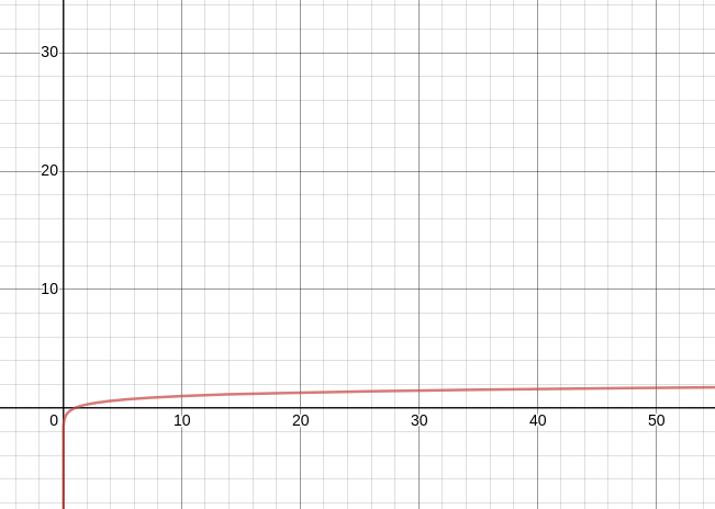
An O(log n) algorithm is considered highly efficient, as the ratio of the number of operations to the size of the input decreases and tends to zero when n increases.
Log linear or quasilinear $\Theta(n. log^k (n))$
If you loop through our binary search $n$ times at most, it’s time complexity would be $O(n. log^k (n))$.
def func(array):
    for num in array:
        binarySearch(array, num + 1)
$O(n. log (n))$ performs better than $O(n^2)$ but not as well as $O(n)$.
Exponential $\Theta(k^{poly(n)})$
$O(2^n)$ means that the time taken will double with each additional element in the input data set. $O(3^n)$ algorithms triple with every additional input, $O(k^n)$ algorithms will get k times bigger with every additional input.

Very poor for large values of n.
So, if $n = 2$, these algorithms will run four times. If $n = 3$, they will run eight times (kind of like the opposite of logarithmic time algorithms).
i = 0
while (i < pow(2, n)):
    i += 1
Runtime will be $2^n$, here the algorithm will run (for n = 3) $2^3$ = 8 times
Factorial $\Theta(n!)$
$O(n!)$ involves doing something for all possible permutations of the $n$ elements.
One classic example is the traveling salesman problem through brute-force search. Traveling salesman problem: “Given a list of cities and the distances between each pair of cities, what is the shortest possible route that visits each city and returns to the origin city?”
Extremely poor running time.
Amortized Analysis
Vectors in C++ are dynamic arrays (like Lists in python), and they are assign memory in blocks of contiguous locations. When the allocated memory falls short, the vector copies the elements in a new memory block with a larger size and then adds the new element.
If we look at the Big-O for pushing a new element, it would be $O(n)$ as with Big-O we consider the worst case, i.e. copying the vector to a bigger memory block, right? But it’s really $O(1)$ amortized. Let’s see what this means.
The motivation for amortized analysis is that looking at the worst-case time per operation can be too pessimistic. So, we think of it as if the cheap operations with $O(1)$ can be considered as two operations, one for the runtime of actual operation and the second one we store in our piggy bank. When we reach the expensive operations (say with $O(n)$ complexity), we can afford it with the runtime allowance stored by other operations.
Suppose, it takes 1 ms to push a new element in our vector. And when we push a new element when the allocated memory to the vector is full, it would take $n$ ms to copy the elements in a larger memory block, where $n$ is the size of initial vector. So, if assume it takes 2 ms to push each element into the vector (even though in it takes 1 ms), and save up this extra 1 ms in our piggy bank each time, then when the times comes to copy all elements, we could pay for it with the ms stored in our piggy bank, which would be exactly $n$ ms as it would take $n$ operations to reach the stage when we have to copy. Now, we can say every push to a vector takes 2 ms amortized.
The motivation for amortized analysis is that a worst-case-per-operation analysis can give overly pessimistic bound if the only way of having an expensive operation is to have a lot of cheap ones before it. Note that this is differentfrom our usual notion of “average case analysis”: weare not making any assumptions about the inputs being chosenat random, we are just averagingover time.
Calculating Big-O
- How to combine time complexities of consecutive loops?
for i in range(n):
    # O(1) operation
for i in range(m):
    # O(1) operation
Time complexity = $O(n) + O(m) = O(n + m)$
If n is around the same order as m, then time complexity would be $O(2n) = O(n)$
- How to calculate time complexity when there are many if, else statements inside loops? Worst case time complexity is the most useful among best, average and worst. So, we look at the worst case, i.e. when if-else conditions cause maximum number of statements to be executed.
For our linearSearch example, we consider that the element is not there at all or is at the end of the list. So, the time complexity would be $O(n)$ even though in some cases it find the element at the start and it would be $O(1)$, but as we consider the worst case we say the linearSearch algorithm has time complexity of $O(n)$.
- A good trick is to double the value of
nand see how the runtime changes.
def func(array: [int], lenArray: int):
    for i in range(lenArray):
        for j in range(10):
            array[j] += 1
    return array
For n where n = lenArray, the loop runs $n * 10$ times.
For twice the value of n , the loop runs $2n * 10$ times. Similarly for 3n, $3n * 10$ times. The runtime increases linearly with n. Hence, $O(n)$.
- Look at the conditions in a loop: $log(n)$
for (int i = 1; i < n: i *= c) { // loop1
    // some O(1) operations
}
for (int i = 1; i < n; i /=c) { //loop2
    // some O(1) operations
}
For loop1, i = 1, $c$, $c^2$, $c^3$, … $c^k$, where $k$ is the number of times loop ran (runtime complexity).
So, as per the condition i < n, the loop stops when $c^k >= n$.
Which gives, $k = log_c^n$.
Similarly for loop2, $k = - log_c^n$ viz $O(log n)$, (ignoring constants!)
How to improve time complexity?
- Improve algorithm.
- Look for redundant calculations.
- Use data structures with better runtime characteristics.
- Reduce the number of constant operations, if possible. This will not change the Big-O of the algorithm but will improve the runtime.
“Premature optimisation is the root of all evil”
The real problem is that programmers have spent far too much time worrying about efficiency in the wrong places and at the wrong times; premature optimisation is the root of all evil (or at least most of it) in programming.
Donald Knuth